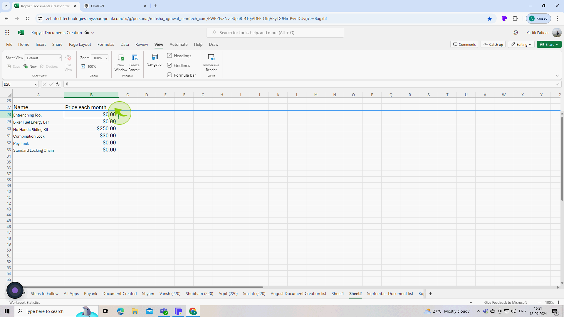
How to freeze a row in Excel ?
|
 Excel
|
Sep 12, 2024
|
5 Steps
Learn how to freeze rows in Excel to keep them visible while scrolling through your data. This handy feature allows you to maintain context and easily reference headers or important information as you navigate your spreadsheet. This document will walk you through the simple steps to freeze rows and enhance your Excel experience. Whether you're working with large datasets or complex spreadsheets, freezing rows can significantly improve your productivity and efficiency.
How to freeze a row in Excel ?
|
 Excel
|
5 Steps
1
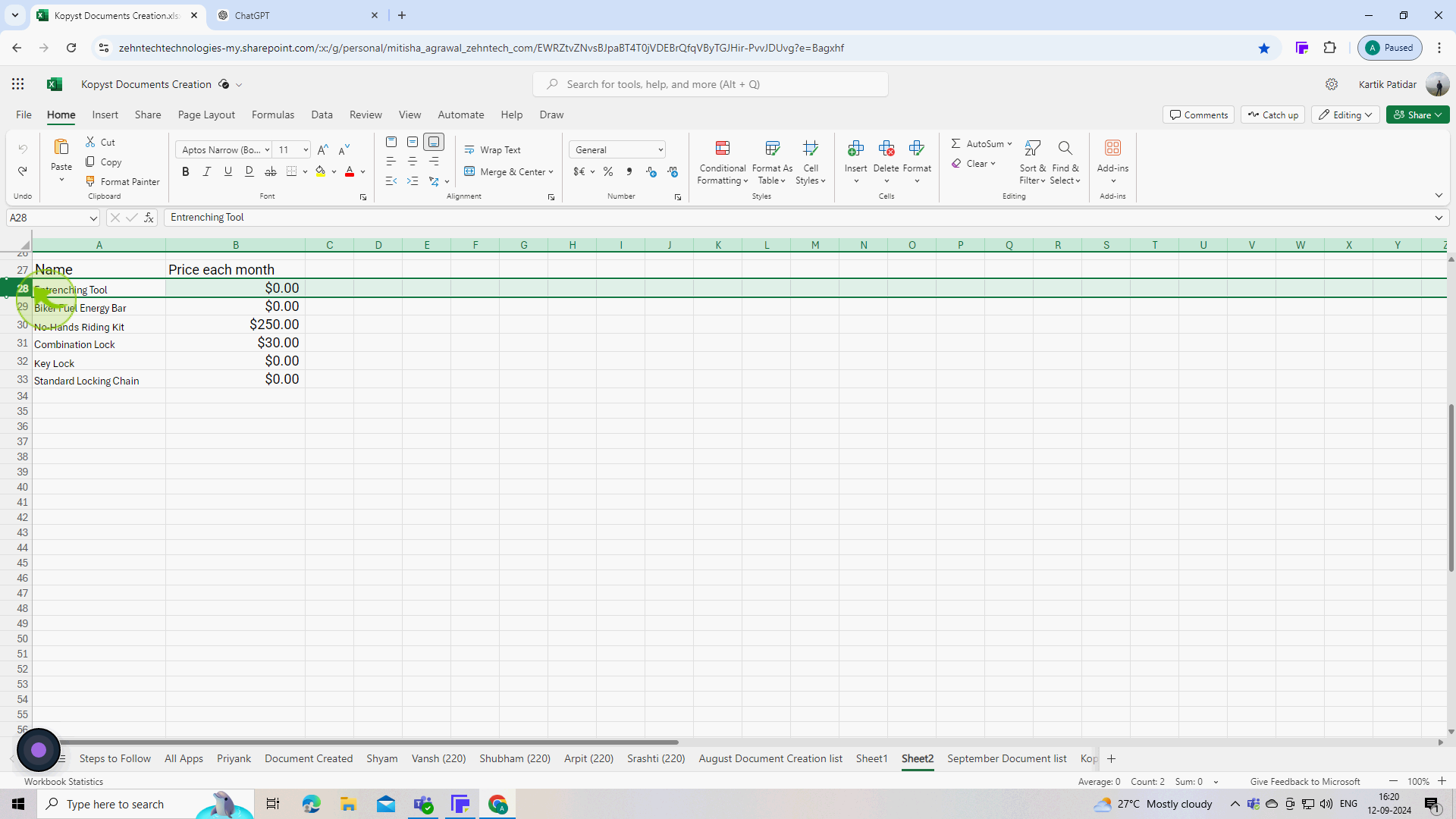
Select the "Row"
Click on the row number directly below the row you want to freeze. For example, if you want to freeze the first row, click on the number 2 to select the entire second row.
2
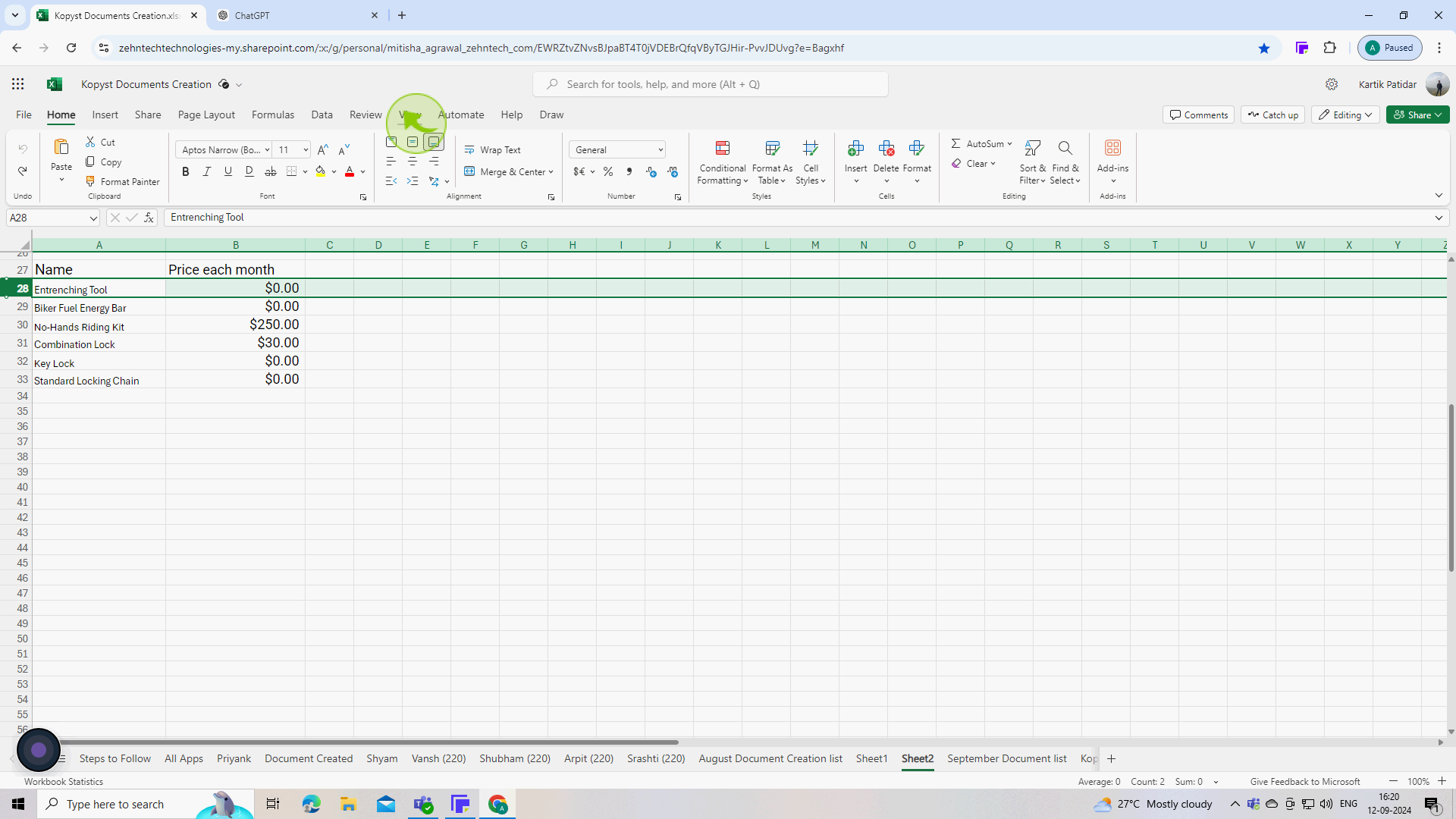
Go to the "View" tab
Navigate to the view tab in the ribbon at the top of the excel window.
3
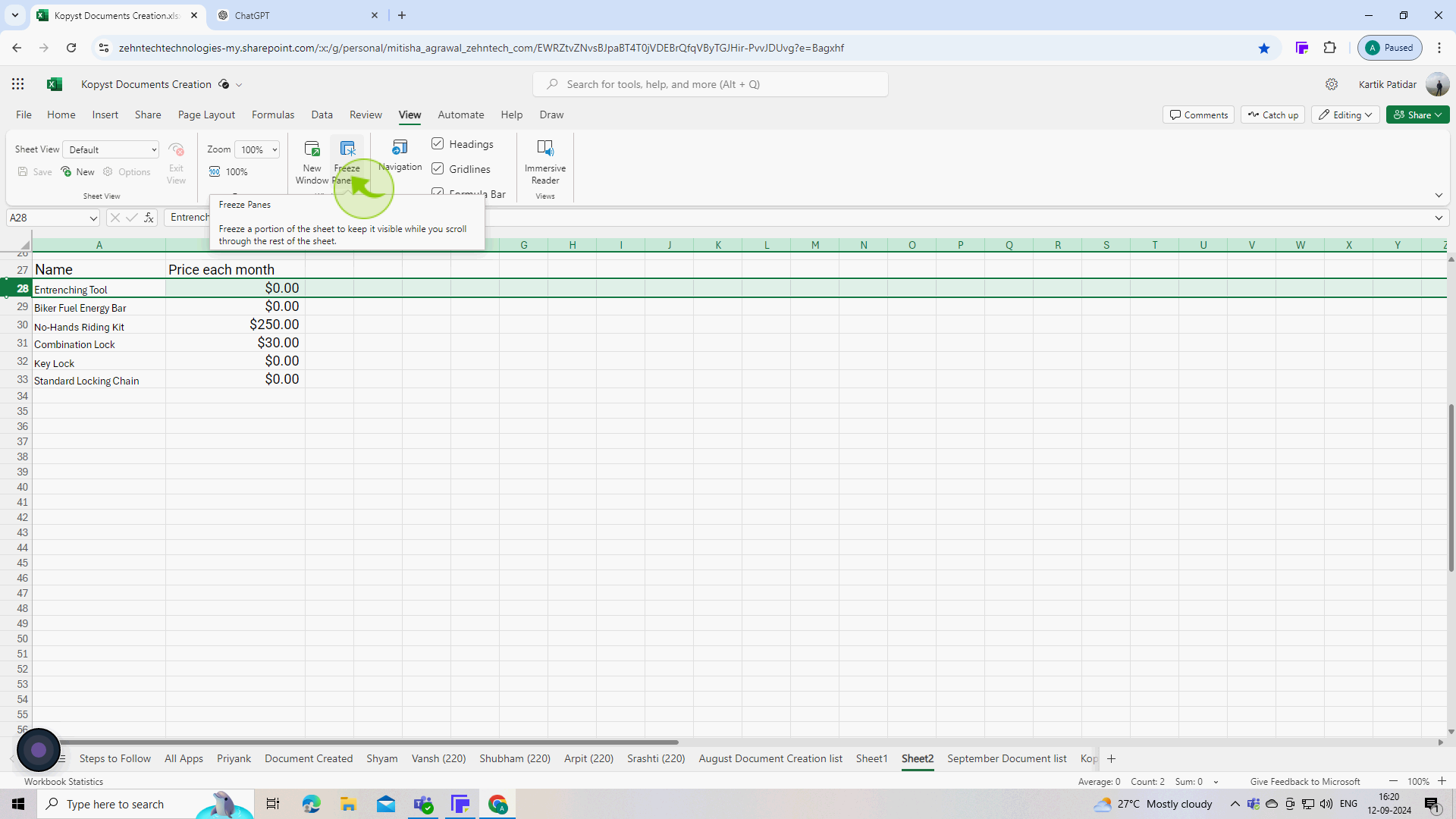
Click on the "Freeze Panes"
In the window group, click on freeze panes then dropdown menu will appear.
4
Choose "Freeze at Selection"
From the dropdown menu, select freeze at selection this will freeze the rows above the selected row. alternatively, if you only want to freeze the top row, you can choose freeze top row from the dropdown menu.
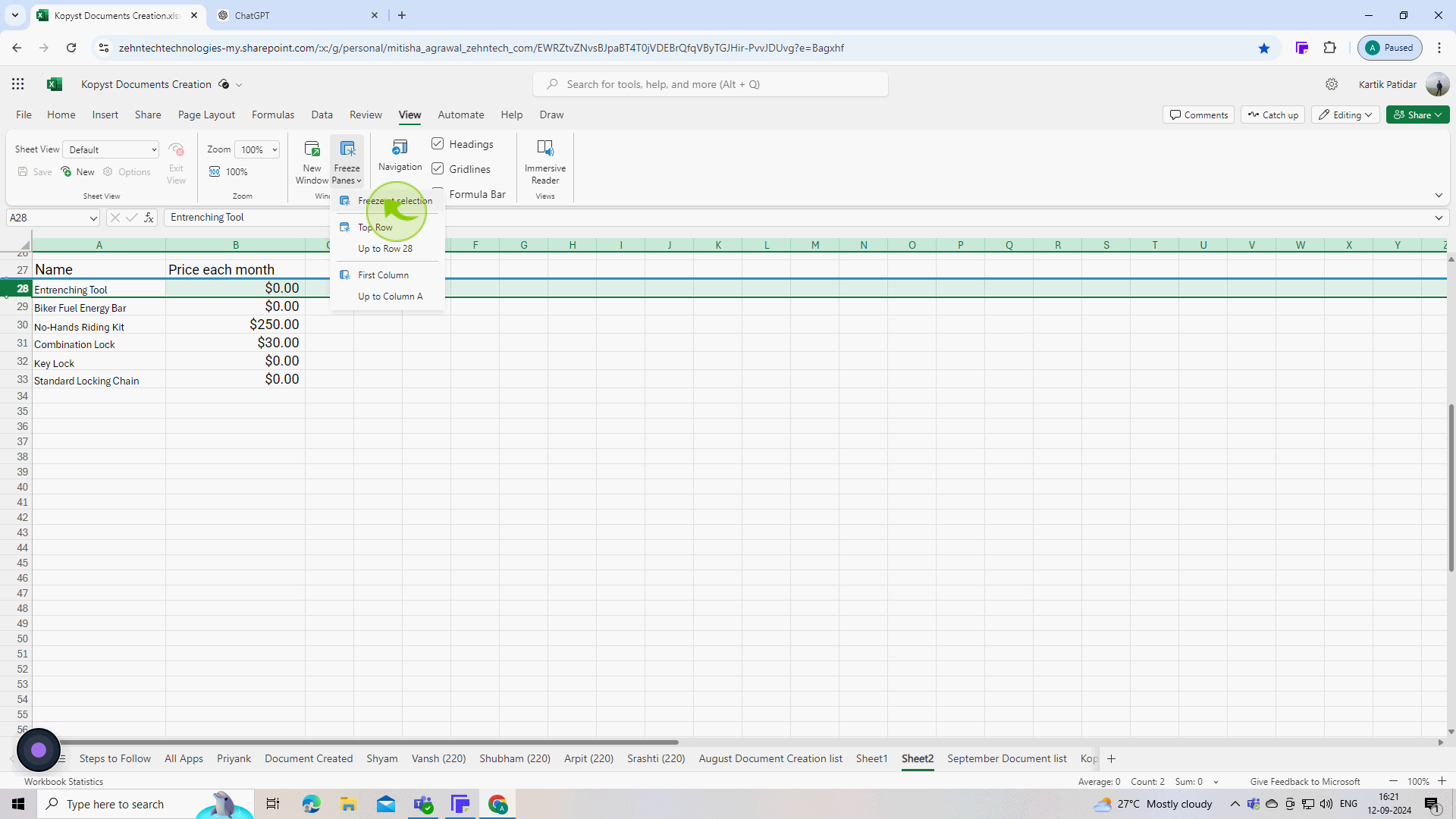
5
Confirm the "Freeze"
You’ll see a thin line indicating that the row is frozen. now, as you scroll through your worksheet, the frozen row will remain visible.
