How to use vlookup in Excel ?
|
 Excel
|
Sep 16, 2024
|
6 Steps
Unlock the power of VLOOKUP in Excel! Learn how to effortlessly find and retrieve specific data from a table or range. This step-by-step guide will teach you the essential steps to use the VLOOKUP function effectively, including understanding its arguments, setting up your data, and applying the formula correctly. Whether you're a beginner or looking to enhance your Excel skills, this tutorial will empower you to streamline your data analysis and save valuable time.
How to use vlookup in Excel ?
|
 Excel
|
6 Steps
1
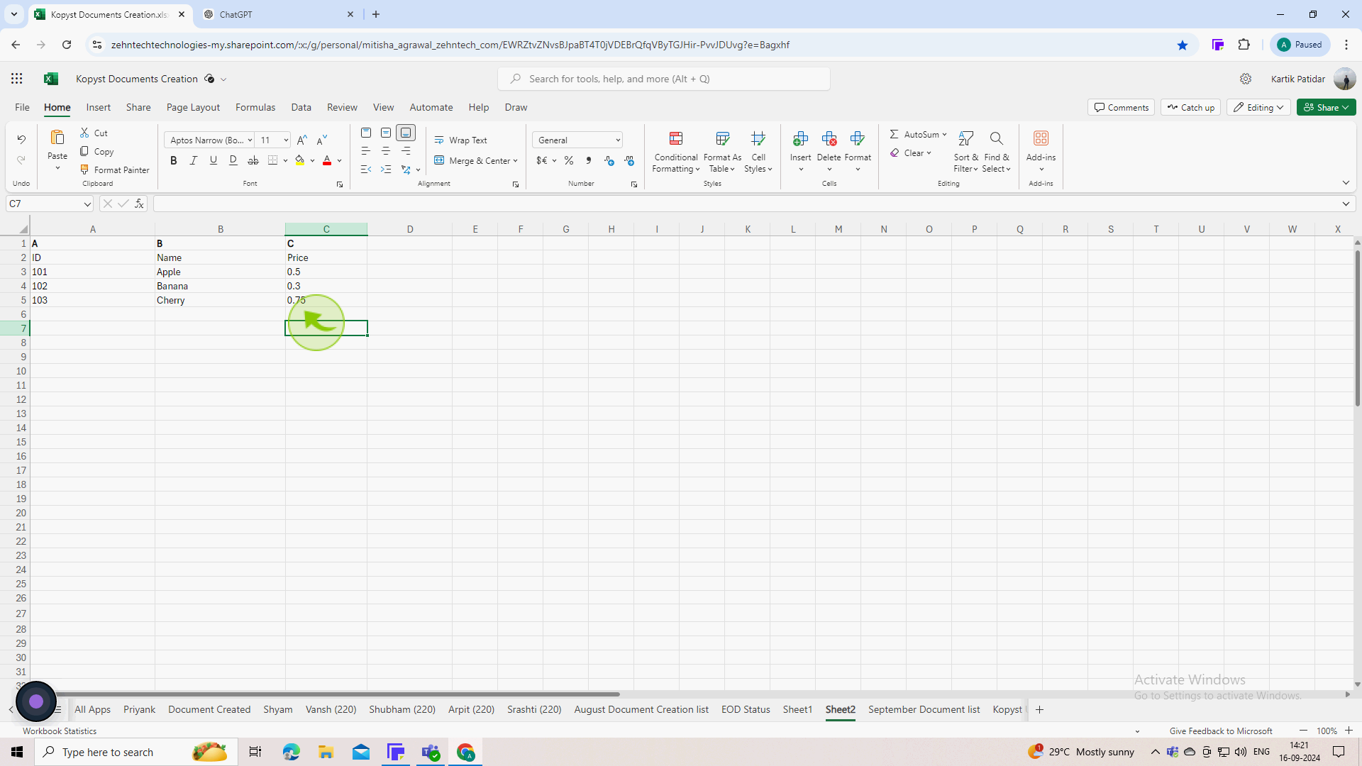
Open "Microsoft Excel" and organize your data into a table format.
Make sure your data is arranged in columns.
2
Click on the "Cell" where you want to display the result of the "VLOOKUP" function.
This cell will show the value returned by the VLOOKUP formula based on your search criterion.

3
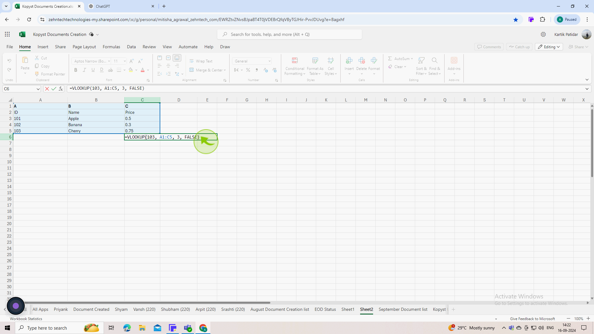
Type the "VLOOKUP" formula into the selected cell.
The basic syntax for the VLOOKUP function is : =VLOOKUP(lookup_value, table_array, col_index_num, [range_lookup])
4
Replace the "Parameters" in the formula with actual values or cell references.
If you want to look up a value in cell C6, you could write: =VLOOKUP(E1, A1:C4, 3, FALSE)

5
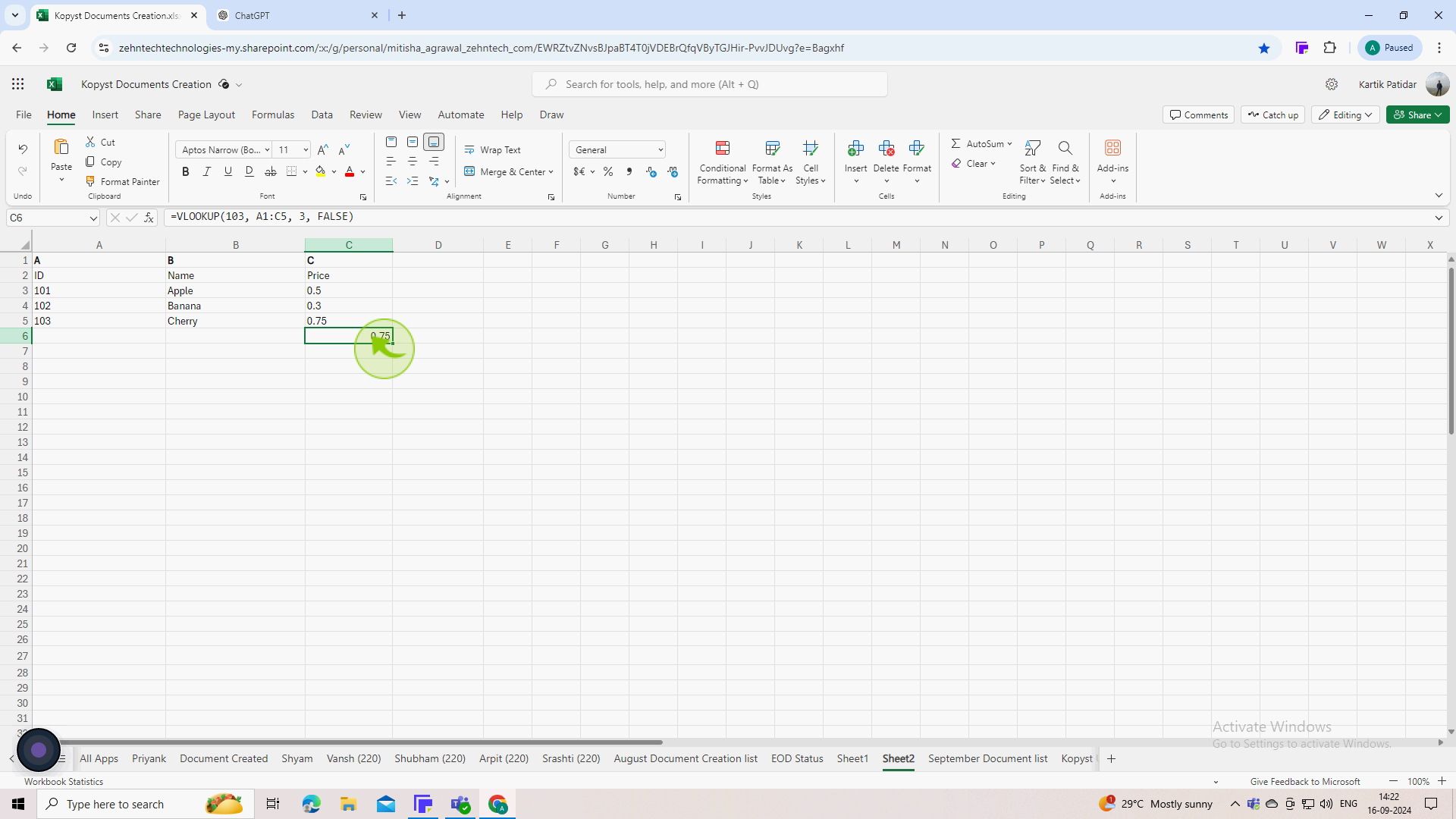
Press "Enter" after typing the formula.
Excel will execute the VLOOKUP function and display the result in the selected cell.
6
Check the "Result" displayed in the cell to ensure it matches your expectations.
If the result is #N/A, it means the lookup value was not found. If you see #REF!, it indicates an issue with the column index number or table array.

